Extreme thoughts

Some thoughts on extreme values, useful for signal detection and R&D management, but often misused by those who don't understand them.

Inspired partly by the writing of my next book (on technology) and by rampant misuse of extremes to make statements about the mean, especially in the cesspool that is IQ-twitter, here are some thoughts on extreme values. TL;DR:

1. There’s a complicated relationship between extreme draws of a distribution and its mean.

2. Because of the statistical properties of extremes, option-valued processes (like basic research) should prioritize a variety of approaches, other things being equal. This suggests that research will benefit from tolerance of a diversity of thought processes and unconventionality. Many companies copy the visible parts of unconventionality, in décor and dress code, while failing at the thought parts.

3. Extremes can give information about the distribution under very strict assumptions, and generally people who use extremes to say things about the mean either ignore those assumptions or expect others not to notice the error.

We’ll consider only the maximum, but the other order statistics (maximum, second largest, third largest, etc, all the way to smallest) are similar.

Extremes are their own thing!

Let’s say we’re given free rein to choose a team of researchers to create and develop a new mode of transportation for urban environments:

The creative process allows us to pick the best idea of these researchers, so what we care about is the maximum value, not the average value, of the ideas.

To simplify, each researcher only has one idea; some have good ideas (to which we’ll assign a positive value), some have not so good ideas (negative value). Most of the ideas will be incremental on what we already have, therefore their values will be close to zero, while a few may be potentially very good

or very bad

There’s a lot of confusion about implications of extremes and implications of means; we will separate them here by comparing the extremes in a number of cases all from populations with the same mean. (The “population” here is the value of the ideas created by the researchers, not the ideas nor the researchers.)

For simplicity, we’ll assume that the value for these ideas is normally distributed, with mean zero and some standard deviation. (We use the standard deviation instead of the variance as our reference “spread” quantity because it’s in the same units as the value itself, while the variance is in units of value-squared.)

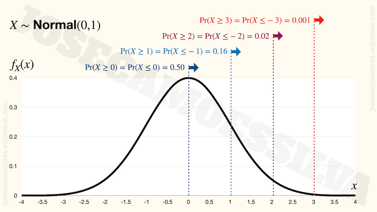
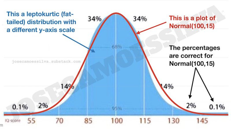
On the off-chance that readers haven’t seen a Normal distribution or are unaware of some of its more relevant implications, here’s one (a real one, plotted not drawn, unlike the ones in many “memes”¹):

Onward to the maximum! We can use e.g. the R programming language to simulate having different teams of the same size; example, for a team of size 10:

rnorm(10)

meaning “draw 10 random numbers from a normal distribution,” with the result

-0.15540263 0.38592374 -0.87592238 0.68691078 0.71727891 -0.34413760 -0.33682228 1.04352354 0.08897479 0.80605669

And we can use the built-in maximum function to find the best:

max(rnorm(10))

This gives us one instance of the maximum of a team; SD = 1 by default. Let’s get a few instances just to have a feel for the issues coming up.

The first column of the next figure has ten of these instances, basically ten teams of ten researchers and the value that we would get for the maximum (of the ten random draws) for each of the teams:

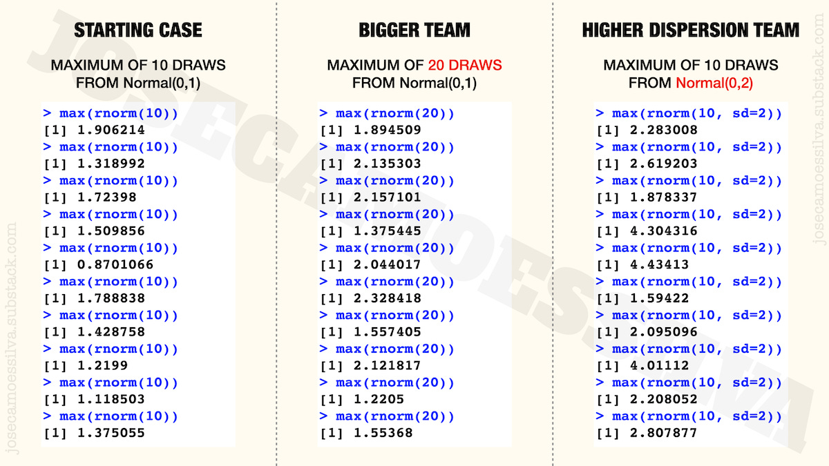
As we can see, there’s some variability even though the teams are all made of 10 researchers and each researcher has the same distribution of value as the others (Normal with average zero and standard deviation one).

If we had a team of 20 researchers, we would get results like those in the middle column: most of them are higher than the values of the first column (with 20 people there’s more chance of getting a high value) but not all of them: the penultimate value on the middle column is smaller than several values in the first column: the larger size doesn’t guarantee a higher maximum.

The last column shows the effect of getting researchers with greater variability of ideas (which translate to a higher standard deviation of their value). This means that there’ll be some completely insane ideas, but also some brilliant ideas; and since we’re picking the maximum, we don’t care about the insane ideas, so we get to have typically higher values. (Again, not all of them are higher than all the other cases, but most are, for reasons that the next figure will make clear.)

We can use probability theory to derive and plot the distributions and the expected values of the maximum for those three cases²:

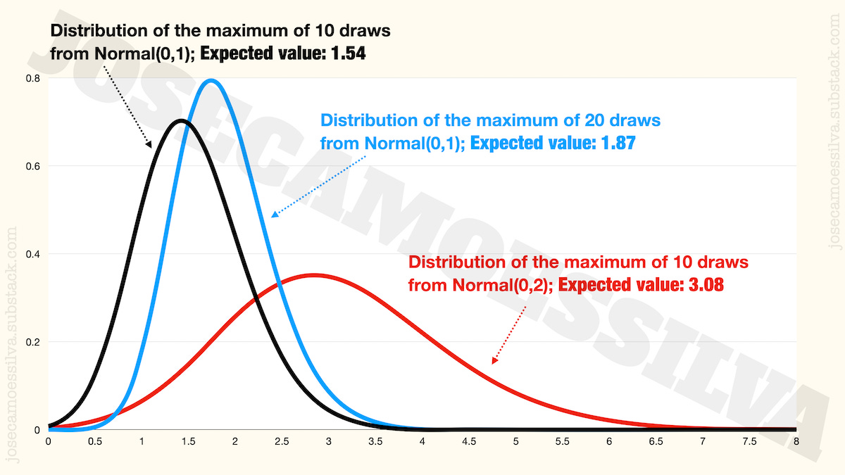
From this toy example, we can already note two things:

First: on average (technically, in expectation) the maximum increases with sample size and with standard deviation.

Second: increases in sample size alone narrow the distribution of the maximum (compare the blue and black peaks); while increases in standard deviation alone spread out the distribution of the maximum (ditto for red and black peaks).

This gives us some ideas on how to staff teams for creative work.

Creativity 101: embrace the weird (yeah, right!)

“The reasonable man adapts himself to the world; the unreasonable one persists in trying to adapt the world to himself. Therefore, all progress depends on the unreasonable man” — George Bernard Shaw.

Modern technological societies recognize the importance of creativity and basic research for the continuing progress, which is why they fund (for now…) research labs and open-ended research and give incentives for private companies to fund research of their own (not just product development).

And yet, one of the most key aspects of creative research, the tolerance of differences and “weirdness” in thought processes is under attack from various sides, some of which seem to mistake weird behavior and weird clothing for actual differences in mindsets and approaches to problem-solving.

But let’s start with the positive side of creativity and think how we’d ideally staff a research team. We’ll just focus on the early part of the product development processes: getting something to work.

The development process has later phases that make sure products will work reliably with average people in the outside world (not just occasionally and for experts in a lab) and can be produced economically at scale. But, in the early parts, creativity is more important than those pesky engineering and business concerns, so we’re going to assume our objective is to maximize the value of the idea that gets turned into a proof-of-concept (or technology demonstration):

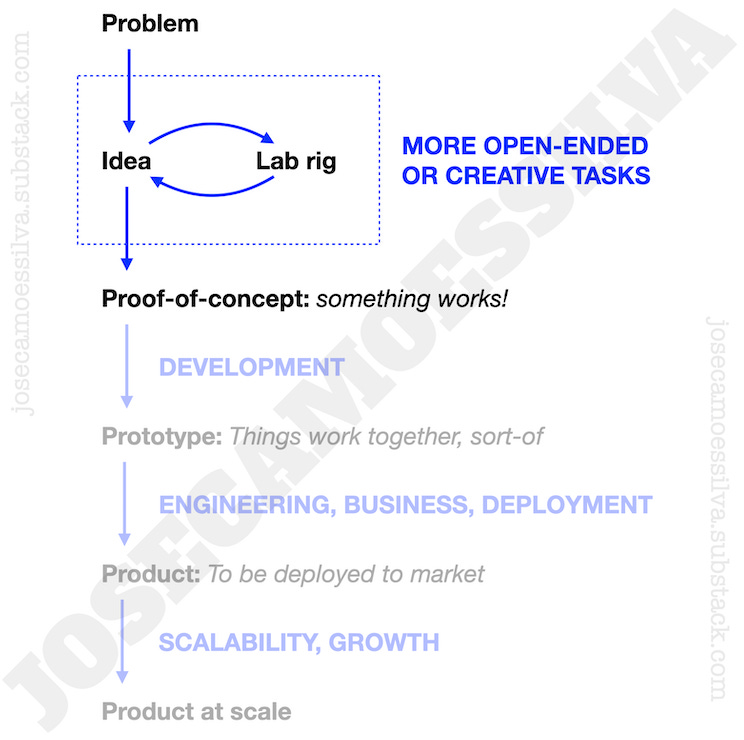
(Image adapted from my book-in-progress on understanding technology. Due to a number of personal and work-related issues, “in progress” is currently aspirational.)

As we’ve seen above, the maximum increases with variation (the standard deviation) and the size of the sample of ideas. (It also increases with the mean value of ideas; we kept that at zero above, and will keep it here as well, since with independent draws that just adds a constant to the result — really, that’s all it does.)

Let’s say our team can generate (and test) 100 ideas per period; here’s how the maximum value of those ideas is distributed for different levels of variation (SD) in the value of each individual idea:

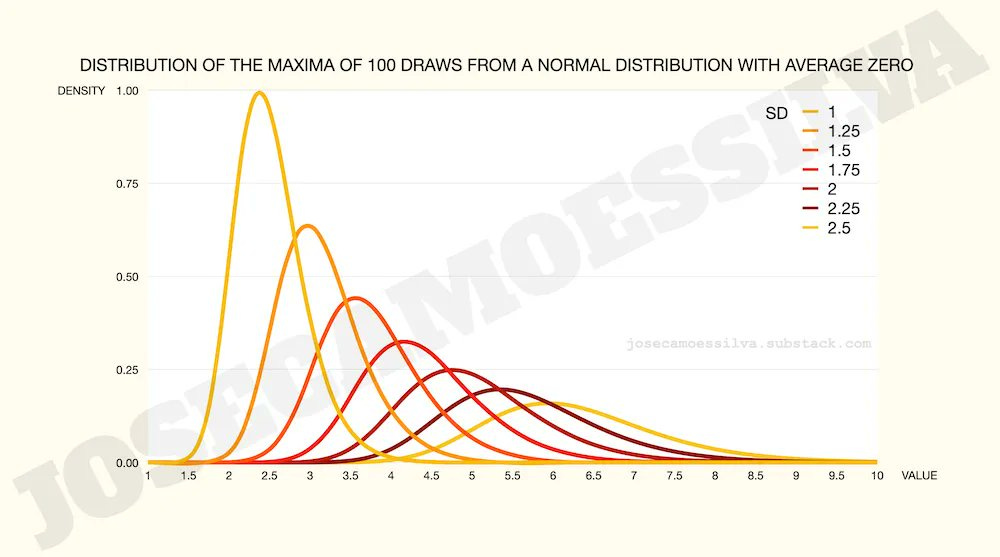
All other things equal (ceteris paribus, for people who like to use Latin phrases to obfuscate simple concepts), management should endeavor to maximize the potential variation in ideas (presumably in a way that maps to value).

Alas, maximizing variation, treated in models as uncertainty and usually assigned the valence of risk (which it isn’t when we’re picking the maximum, but it is when evaluating a single investment), is the opposite of the training most managers receive.

And large institutions have a bias towards conformity, as many many oh so many studies of organizations have shown (back when people who researched business technique and management thought studied organizations for practical purposes instead of writing treatises on theoretical sociology and the evils of capitalism).

We’d think that the “nerd culture” that has become more popular with the financial success of computer geeks would have dealt with that conformity culture, but it just moved the conformity to another set of visible symbols (associated with the hitherto “weird” thinkers), in what marketers and public relations people since the late 1800s would call identity-building and modern political science discourse calls performative.

In other words: nerdy clothes, hobbies, and references (often wrong); stated preference for STEM and STEM-adjacent entertainment properties (revealed preference orthogonal if not opposite); awkward behavior around others (mostly performative, though rudeness is usually real); and above all conventional thinking and risk-averse incremental-when they-have-them ideas.

And at a corporate level, avant-garde décor (equal to that of everyone else who’s also trying to “be different”), impractical but novel corporate practices like hike meetings and floating desks (meaning that people move all their stuff with them, not that desks float in space with no supports), many other pointless fads that have little productivity impact, and —of course— “no hierarchy,” which means the hierarchy is clear and well-understood by any insider who isn’t a total doofus, just not formally indicated in a way that outsiders could catch at a glance.

But that’s okay for many institutions, because differences in mindset aren’t visible in photo-ops and B-roll for CEO interviews, but hike meetings and sleep pods are.

Signal detection: the good, the bad, and the ugly

Taking the opposite direction, what can we learn from extremes? In other words, if we observe a random value that falls to the extreme side of a distribution, what can we conclude from it?³

The good: if we know the properties of the distributions we are comparing, a draw from the extremes may be more informative than one close to the mean.

Engineers (especially the superior type of engineer, EECS 🧐) call this signal detection: when we observe one draw from one of two close distributions, if the value is near the mean of those distributions (assumed to be close in mean and with the same SD), it’s very difficult to tell which of the distributions it came from; but if it is far from the mean, it’s much more likely to come from one of them than from the other:

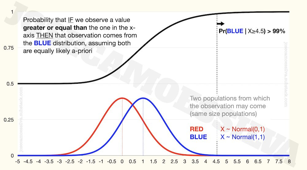
What this means: if we’re trying to determine which of these two distributions a random draw comes from, and we observe a value that is greater than 4.5 (it passes a filter that eliminates any observation with X < 4.5), then we can be 99% sure that it came from the blue distribution.⁴

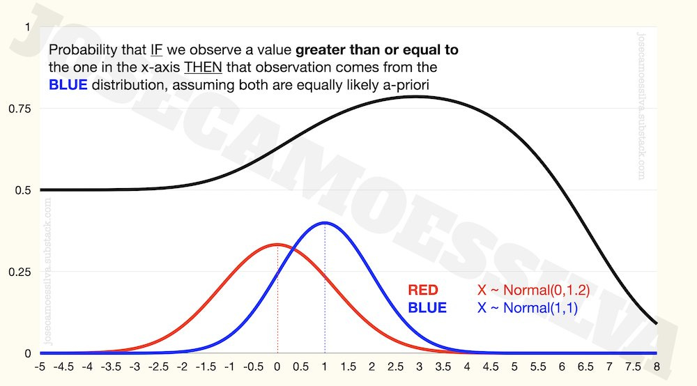
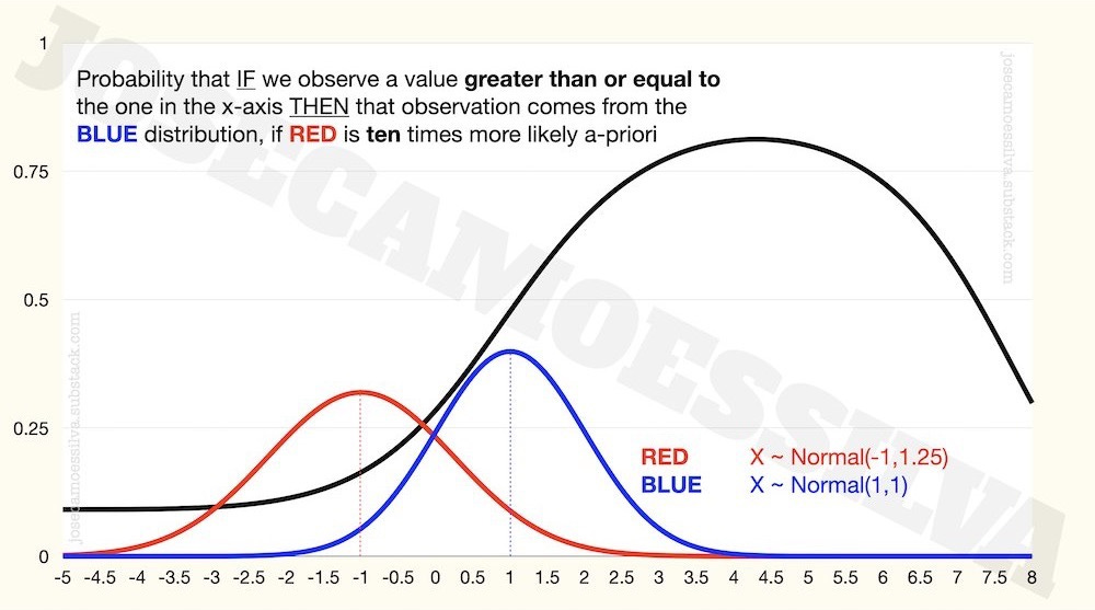
The informativeness depends on all parameters, so when we have a larger population for one of the distribution or one of the distributions has higher variation, the clean result above no longer applies:

The bad: using maxima (and other extremes) to make assertions about population differences, particularly the means of those populations, without taking into account different population (or sample) sizes and differences in standard deviations.

As we saw above, the maximum depends also on the size of the sample/population and the standard deviation; with some minimal tweaking we can find combinations of these that mimic a shift in the mean of the distribution; for example,

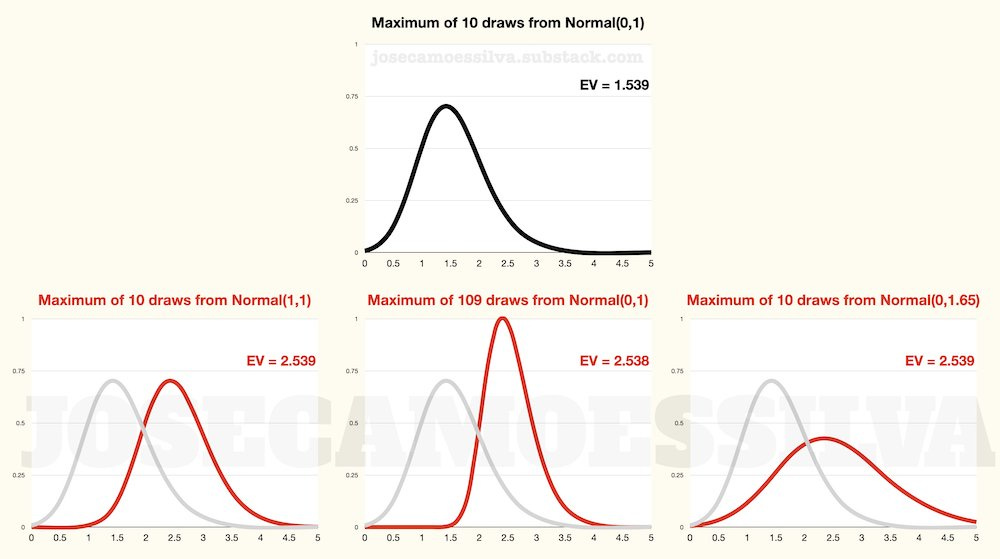
So, when we see that the best powerlifter from Gym B has a combined score of 2.54 (say bench press divided by bodyweight) while the best powerlifter from Gym A only has a score of 1.54, the bad conclusion is to use that as support for Gym B having a better average powerlifter than Gym A.

As the bottom row in the figure show, Gym B having many more powerlifters or having powerlifters with more variability in scores while having the same average as those in Gym A are also possible explanations.

In many real-world situations, different effective population sizes (due to availability of gyms, for example) tend to be the most likely explanations for large discrepancies in extremes. And as we’ve seen above, small differences in standard deviations can make big changes to the distribution of the maximum.

Which bring us to:

The ugly: using these bad inferences to make political points or to demean groups of people, usually furthering the error by then applying what would at best be population-level results —had they been correct— to individuals.

Random draws at the tail can be informative (with a lot of assumptions), but extremes by themselves are unrepresentative of mean differences, as per the bad above (the sprinters in the double-quoted tweet are competitive runners, and in a competition the winners are by definition the extremes).

For information about means we need random samples.

1. It’s not difficult to plot distributions, but why care about accuracy when you can just use a drawing tool? Gahhh! For added irony, IQ-based “memes” regularly use this:

2. The probability that we observe a particular value x for the maximum of N draws is given by the joint probability of observing one of x and N-1 values lower than x, times the number of variables (the size of the sample) that can take the value of x,

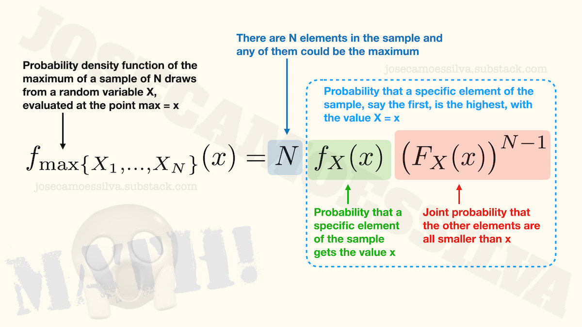
Because of the properties of the Normal, we need to use numerical methods to approximate the cumulative density function (the capital-F function) and to compute the expected value.

All figures in the post were plotted from R results (on Keynote) but according to my sources —I wouldn’t soil my hands with it 😉— Microsoft Excel has both the probability density function (the f(x)) and the cumulative density function (the F(x)) for the Normal distribution (among others) as predefined functions. Alas, it doesn’t do the numerical integration needed for the expected value.

3. Yes, I know I overuse that spaghetti western title. There's almost always an opportunity to use this old favorite across many fields, as many people use tools and principles correctly, incorrectly, and uglily. (Yes, it's a word.)

4. The greater-than-or-equal-to approach is a cope for the use of continuous variables; there’s an analytic result for the probability density functions that shows the same thing, but some people don’t like to do/see actual math, so here it is footnoted in its elegant entirety:

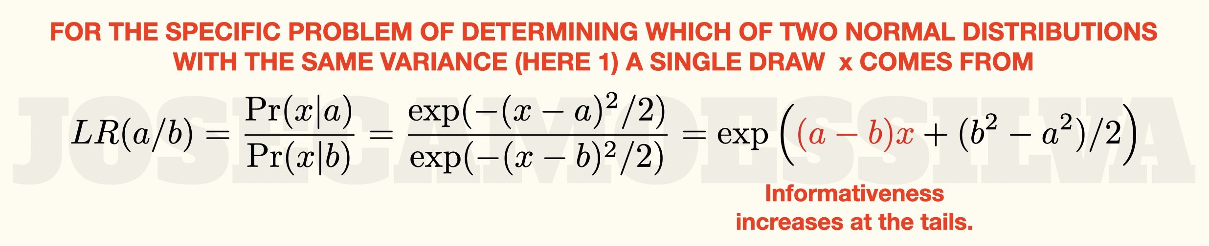
(For other values of the variance, with the same value for both distributions, just divide the argument of each of the exponentials by that same variance.)

The likelihood ratio (the probability that we observe the data conditioned on the distribution) is only a component of the final probability, it needs to be Bayes-formula-ed with the prior distributions to get the posterior distribution.