
Populations, proxies, and precision
Populations, proxies, and precision
Three common errors in data analysis, especially on social media.

A half-Feynman post: three easy things (that many people get wrong).

This post was written over a long period, inspired by many repetitions on social media of the errors illustrated here, with particular incidence in IQ-twitter.
Distributions versus individuals
Every so often I (JCS) ponder writing a post called “IQ: the good, the bad, and the ugly.” (It won’t happen, because I don’t want to wade into that cesspool.)
The good would be that IQ tests supposedly give smart poor kids a chance against the stupid rich kids in university admissions;1 the bad —and there’s a lot of it— would be those people who talk about IQ because they believe it makes them appear smart (while what they say proves the opposite); and the ugly —and it’s very ugly— would be the people who like to use IQ as a veneer on their… let’s call them preconceived notions about demographic groups.
Essentially the ugly side is just a highly visible example of a common problem of thinking with distributions: the notion that the distribution of some quantity in a large population can be used to make useful assumptions about individuals either by themselves or in paired comparisons.
If we assume for argument sake that there are differences between populations along the lines of some commonly cited, those differences aren’t useful for individual assessment or for paired comparisons, as can be shown by the overlap between the curves in the top panel of the figure below; also illustrated by 4000 draws from each distribution (bottom panel).
The blue distribution has average 0 and standard deviation 1; the orange distribution has average -1 and standard deviation 1. As the bottom panel illustrates, there’s plenty of overlap at the individual level (the vertical dimension is for separation only).

A common argument is that in a paired comparison blue is expected to be better than orange: that’s a statement about the averages, not individuals. Furthermore, we can calculate how often that will happen at an individual level. That is, comparing two random draws, one from each of these distributions, how often will the draw from the blue distribution be larger than the draw from the orange distribution? Absent additional information, this happens 76% of the time.2
Therefore, in 24% of the cases, using the expectation is wrong. Since humans have a tendency to look for confirmatory evidence instead of neutral information (fallacious reasoning, but that’s what we all do), in those 24% of cases people will discount additional evidence that would make the error visible.
“Why don’t they just leave the old variable in there too?”
There was some recent [at the time of writing, not publication] agitation on Twitter about a change in a medical diagnosis procedure where a demographic variable was replaced by more detailed individual information. The question raised by those agitated was the one above: why not let that variable stay in the model? Overwhelmingly the suspected answer was political or social pressures overruling science.
But there’s an actually good reason to avoid having highly related variables in a model: it’s called multicollinearity. (Linear algebra strikes again!)
To avoid the emotionally-charged and historically problematic variable, we’ll use the following hypothetical example:
There’s a condition that causes early hair loss in people who have it.
There’s a gene associated with that condition, gene EHL; if someone has the gene there’s 99% chance they’ll develop the condition; if they don’t have the gene, there’s 99% chance they won’t develop the condition.
90% of Spaniards have that gene, and 10% of Portuguese have that gene.
Until gene testing for EHL was available, doctors observing the first signs of early hair loss would make the decision to prescribe FollicleGrow2000 treatments based on whether the patient was Portuguese or a Spaniard. This led to some misdiagnoses and the occasional Spaniard with very long and bushy eyebrows (a side effect of FollicleGrow2000 if the patient doesn’t have the EHL gene) and some prematurely bald Portuguese.
Once medical science has developed a test for the EHL gene, knowing whether Jorge is a Spaniard or Portuguese, given that we know whether Jorge has the gene, is of no help: If Jorge has the gene and is Portuguese, his likelihood of having early hair loss is 99%, (and the Portuguese part adds nothing to it). If Jorge doesn’t have the gene and is Spanish, his likelihood of having early has loss is 1% (and the Spanish part adds nothing to it).
It would appear that once we have information about the gene, we don’t need the country.
But it’s actually worse. Because if we create a model where two independent (or right-hand-side) variables (country and gene) are closely related, then the statistical tool that measures their effect on the dependent variable (whether someone should get FollicleGrow2000) becomes unstable and returns sub-optimal or nonsensical values.
Basically, the statistics work by trying to allocate variation in the dependent variable to the independent variables; but because the independent variables have such close correlation, there are many different allocations that produce the same results on the dependent variable; so, sometimes the coefficients for these closely correlated independent variables are determined entirely by random factors — like those that make the probabilities in the example above 90% and 99% instead of 100%.
The above was a simplified version of reality because the information carried by the gene test completely negates any additional value of knowing the country; but this is just an example of the more general multicollinearity problem, where adding a proxy A to a model that already has the variable it proxies for, X, creates a statistical estimation problem that can remove the significance (may Bayes forgive us) of both:

In the above example we have an outcome (Z) which is a function of two causes (X and Y) and some stochastic disturbances (things we don’t observe so they’re not included in the model; we assume that their average effect is zero).
In the past, we didn’t have a way to measure X directly, so we used a proxy, A, which is correlated with X (in this example highly correlated, in the real case that got people upset on twitter, moderately correlated).
As we can see, the old model in the example shows both effects of A and Y on Z, and that’s representative of the old model in the real case, with A standing in for the demographic variable.
When we get a way to measure X directly, placing it in the model gives similar results (because A and X were highly correlated; in the real case, replacing the demographic variable with a medical test improves the causality substantially).3
When we include both A and X in the model, the result is statistical — technically linear algebra — mayhem: both drop out of the model (using the frequentist “significance” as the criterion for inclusion, may Bayes forgive us).4
Errors in measurement: a common misconception
In the absence of direct measurement of the desired quantity, proxies allow for model-building, but they raise the issue of error in measurement.
Whether errors in the independent variables (the right-hand-side variables) come from the use of a proxy or from errors in measurement, there’s a common misconception about their effect: that those errors will somehow “even out” just like the stochastic disturbances (essentially the “errors” in the dependent variable).
That’s wrong.
Errors in the right-hand-side variables bias the coefficient of those variables towards zero, i.e. they make the variable appear to have less weight on the dependent variable than it actually does. This is illustrated below.

When we compare the slopes of the best linear fit between the real model (using the X) and the model with errors in measurement (with the tilde-x), we can see that the slope with error is flatter (that is, the effect size is smaller) and we can see why it’s flatter: because the error in measurement “spreads out” the x-axis variable, so to fit the Y to that wider “cloud” the line has to be more horizontal.
For comparison, the stochastic disturbance (the epsilon) is combined with the “undisturbed” Y: it has no impact on the x-axis and its average is zero so it doesn’t change the fit (remember that the fit is measured vertically, not horizontally; it’s the difference between that line and the data points measured along the y-axis only).
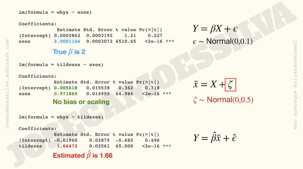
Above is the numerical counterpart of that figure: when we estimate a model of Y on the (unobserved) X, we get the true parameter (not precisely because there are stochastic disturbances, but a frequentist would say that the 2.0001166 is “not significantly different — may Bayes forgive them — from 2); when we compare the true X with the measured tilde-x, we see that there’s some error, but there’s neither a bias (the intercept is 0 —frequentists, non-significant, Bayes forgive them, etc) or scaling (the parameter is 1 —frequentists, non-significant, Bayes forgive them, etc); but when we calibrate a model of Y on the tilde-x we get a significantly different (frequentists, etc) coefficient for the x-tilde (1.66 instead of 2; biased towards zero as expected).5
Sadly, there are still many examples of people (and not only in the social studies fields) that believe —incorrectly— that the stochastic disturbance will take care of any errors in measurement.
And if you believe that, I have a great ocean-side ski chalet for sale in Albuquerque, NM.
This footnote was going to explain how that 76% is calculated, but instead let’s give the hordes who love talking about IQ distributions the opportunity to show that they know something —a very basic something— about probability calculations. Nota bene: calculations, not simulations.
“Substantially” because we’re avoiding the loaded word “significantly,” may Bayes forgive those who use it.
This is the problem of multicollinearity, created here by the correlation between A and X becoming an almost-singular matrix that the program has to invert. Linear algebra doesn’t like to invert almost-singular matrices and the results are as shown: loss of information on a grand scale.
The logic, using formulas:
